Gaussian splatting the latest and greatest in “novel view synthesis”. Allowing you to explore a complete 3D scene, constructed from a limited set of images. These ideas have been popular in photogammetry (google maps) and somewhat recently the machine learning wave produced Neural Radiance Fields (NeRFs).
From Original Gaussian Splatting Paper: Bicycle rendered with Gaussian Splatting.
Gaussian splats are interesting and gaining wide popularity because of the high-quality real time results you can produce. The splats gives us surprisingly fast and beautiful results when compared with the previous state of the art. It’s allowed for a cambrian explosion in research, improving the data, efficiency of the method. Researchers have also applied the method to new areas like SLAM and agential planning and creating new 4D motion synthesis to list a few. You can see an ever updating list of research by following MrNeRF’s Tracking Page.
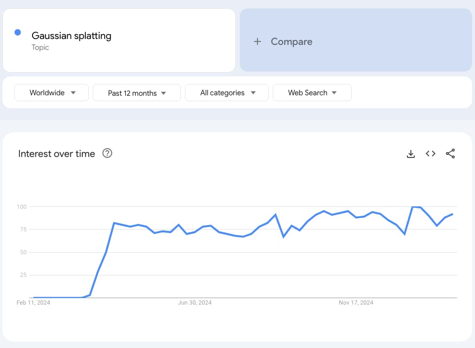
The trend in interest for Gaussian Splatting, spiking with the release of the original paper.
However the math and processes used to create them has been just as fuzzy as the Gaussians in my mind. So I have created this post mostly as an explainer to myself on how the methods work and why certain math tricks are used.
I will outline the basics of the process, the results they give us. And some more minutia around the weirder aspects, for outsiders like me, such as why spherical harmonics ended up being involved.
I have decent linear algebra knowledge and can program well enough to shoot myself in the foot. But I have relatively little rendering experience. So the post will hopefully be approachable to most anyone with a STEM / games-programming background. I am likely to make some mistakes on the explanations though so please reach out to me if you notice any :)
What is a Gaussian and why is being splat?
The main component of Gaussian splatting is the 3d Gaussian. Which is in essence a fuzzy 3D ellipses when rendered. The splatting in the name refers to how each of the Gaussians in the reconstructed scene apply their influence on the final 2D projection. They are projected (“splat”) against a subset of the image. The depth of the projection is preserved though - which does lend to a physical interpretation of multiple paint splats falling against a canvas - with the further splats overlapping the closer. The depth is useful beyond this for depth map purposes too.
Why Gaussians
Gaussians are very useful for the process of novel view synthesis because they are easy to efficiently render, but also very easily differentiable. This becomes important when you are looking to use the powerful techniques that have grown alongside machine learning optimisation.
The efficient rendering of Gaussians should not be overlooked as it provides a massive benefit over NeRF based techniques, by avoiding the expensive ray marching. It is important to note that we don’t just use spherical (isotropic) Gaussians, but rather scale and rotate them (anisotropic) to better fit the training view.
While a few of the Gaussians appear unimpressive, once you scale the number to a few million you are able to see the higher fidelity they give you. Ultimately reproducing clear 3D scenes which high definition and support reflections within the render.
A few thousand Gaussians in the training process. Can you spot the muffins?
Training
The training process is required before you can see any of the millions of Gaussians give you any beautiful results. Similar to most machine learning processes, the Gaussians are moved around and reshaped in a loop, compared against the training images provided. In most cases the training images will usually be the thousands of images taken from a video.
A high level diagram of the training process is shown below, with figures from the original paper, and a very useful overview paper.
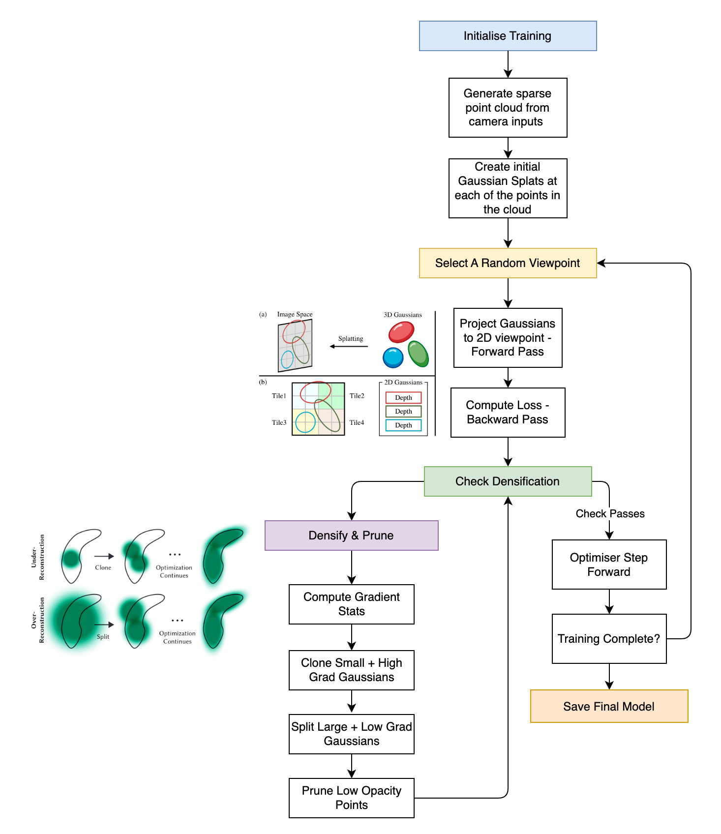
Note that while the technology used for the training is similar to the training for machine learning, no neural networks or transformers are present in the final model or rendering process, unlike NeRFs. This is one of they key benefits to the process in speed and memory usage. We are simply optimising how the Gaussians should be stretched or positioned and which of them should be removed or cloned.
Gaussian Math
Each Gaussian can be represented by four parameters:
- A centre position in 3D space
- A covariance matrix that defines the shape and orientation
- A global opacity value
- A colour value
Altogether the four parameters allow for great flexibility in how each Gaussian impacts the final scene reconstruction. Most importantly though the parameters are tunable when training.
In order to see the impact of a 3D gaussian on the final image though, the 3D gaussian has to be projected (splat!) onto a 2D image. The transform for this process is for each Gaussian :
While this formula might look intimidating, it’s actually modeling something quite intuitive: imagine you have a fuzzy 3D ball (your Gaussian) and you’re taking a photo of it. Here, represents your 3D fuzzy ball’s shape, is how you move the ball into the camera’s view, and is like the camera’s lens - it “flattens” the 3D ball into a 2D oval. The result is the shape of the fuzzy oval you see in your photo. This is why Gaussians appear as different shaped ovals depending on your viewing angle - just like how a ball looks circular from the front but oval-shaped when viewed at an angle!
You can interact with a set of simulated Gaussians in the below. Notice how the 2D image changes how the Gaussians appear on the final splat as the camera moves. In the real training the estimated for these camera positions will come from the initial Structure from Motion (SFM) step.
It is the 2D projection that you see on the right (though with millions more Gaussians), that is then used to compare the positions of the Gaussians against the training images. The final rendered color at each pixel is given by layers the contributions of each Gaussian splat in the projection:
This formula is essentially describing how semi-transparent layers stack, much like painting with watercolors. Each Gaussian acts like a semi-transparent paint splat, where represents how opaque each splat is (0 = invisible, 1 = solid), is the color of each splat, and represents how much you can see through all the previous layers. For example, if you have a red splat with 50% opacity in front of a blue splat with 100% opacity, the final color will be 50% of the red color plus (50% of 100% of the blue color), because you can see half of the blue through the semi-transparent red.
Where:
- is the number of overlapping Gaussians at that pixel
- is the color of the i-th Gaussian
- is the opacity of the i-th Gaussian
Within the paper one key difference is used between the formal definition of the Gaussian and a more efficient approximation. The standard covariance matrix for a 3D Gaussian describes the spread and orientation of the Gaussian within 3 dimension:
Instead of thinking about this covariance matrix as an abstract mathematical construct, we can think of it as a “shape descriptor”. This is why the authors split it into two more intuitive components: scale () and rotation (). It’s like describing an egg - first you say how long, wide, and tall it is (scale), then you say which way it’s pointing (rotation). This is much more intuitive than trying to directly optimize nine interrelated numbers in the covariance matrix!
The original paper authors point out a key issue with this matrix though: covariance matrices are only meaningful when they are positive semi-definite. This is a difficult constraint to add to a gradient descent training loop:
As a result, we opted for a more intuitive, yet equivalently expressive representation for optimisation. The covariance matrix Σ of a 3D Gaussian is analogous to describing the configuration of an ellipsoid. Given a scaling matrix 𝑆 and rotation matrix 𝑅, we can find the corresponding To allow independent optimization of both factors, we store them separately: a 3D vector 𝑠 for scaling and a quaternion 𝑞 to represent rotation. These can be trivially converted to their respective matrices and combined, making sure to normalize 𝑞 to obtain a valid unit quaternion.
Thus when optimising the Gaussian placements the focus is not on a traditional statisticians covariance matrix but instead on the two more easily optimized scale () and quaternion rotation () matrices. Separating the scale and rotation into two separate matrices allows them to more successfully be tuned independently but also neatly side steps the issue of positive semi-definite(ness). The new and matrices are standard three dimensional scaling and rotational matrices which are far easier to work with computationally.
Optimisation Loop
The main target of any optimisation process is the loss function which we would like to minimise. We are mainly interested in taking the same camera positions and images within the data as our training set and comparing them with the output of the rendered 2D projection of the Gaussians. The loss function below shows how a combination the distance between the images and structured similarity are all that is needed. is a tuneable weighting factor, typically 0.2, which weights which measure will have a greater impact.
The important thing to remember is that we are trying to tune the colour, opacity, position, scale and rotation of each Gaussian within the scene. The loss function guides the optimisation ensuring we tune those four parameters for each Gaussian toward the best image quality possible, in theory. In this manner we follow a very similar line to most machine learning training loops, but with specific focus on the rendered output as our comparison.
Some psuedo-python code gives a simplified view of the sizes of the parameters we are tuning and the loss function loop.
class GaussianModel:
    def __init__(self):
        # Initialize parameters with requires_grad=True
        self.means = nn.Parameter(torch.randn(N, 3))
        self.scales = nn.Parameter(torch.ones(N, 3))
        self.quats = nn.Parameter(torch.zeros(N, 4))
        self.opacity = nn.Parameter(torch.ones(N, 1))
        self.colors = nn.Parameter(torch.ones(N, 3))

    def forward(self, camera):
        # 1. Transform Gaussians to camera space
        positions_cam = transform_to_camera(self.means, camera)

        # 2. Compute covariances using scale and rotation
        covs_3d = compute_covariance(self.scales, self.quats)

        # 3. Project to 2D
        means_2d, covs_2d = project_gaussians(positions_cam, covs_3d)

        # 4. Render
        return render_gaussians(means_2d, covs_2d, self.colors, self.opacity)

# Training loop
model = GaussianModel()
optimizer = torch.optim.Adam([
    {'params': model.means, 'lr': 0.001},
    {'params': model.scales, 'lr': 0.001},
    {'params': model.quats, 'lr': 0.001},
    {'params': model.opacity, 'lr': 0.01},
    {'params': model.colors, 'lr': 0.01}
])

for iteration in range(num_iterations):
    optimizer.zero_grad()

    # Sample random training view
    camera = sample_training_view()
    target = load_target_image(camera)

    # Forward pass
    rendered = model(camera)

    # Compute loss
    loss = compute_loss(rendered, target)

    # Backward pass
    loss.backward()

    # Important: Normalize quaternions after gradient step
    with torch.no_grad():
        model.quats.data = F.normalize(model.quats.data, dim=-1)

    optimizer.step()

    # Every N iterations: density control
    if iteration % 100 == 0:
        clone_or_split_gaussians()
        prune_invisible_gaussians()
				step_up_spherical_harmonic_deg()
Rendering
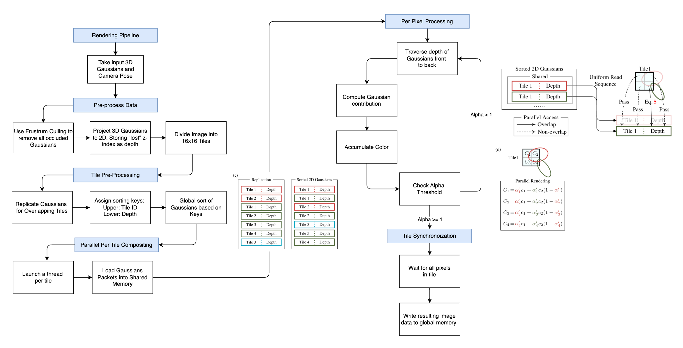
The rendering process is one of the key features of Gaussian Splatting. It operates with less memory requirements compared with NeRFs, and is able to render in real-time. An overview of the rendering process is shown below, highlighting how the data is split for parallel processing on the GPU.
Spherical Harmonic Lighting
Spherical harmonics are definitely a surprising bit of math to pop up in the world of rendering, especially if you throw the term casually into google you’ll find it’s deeply nested in the quantum mechanics world.
Not to worry though, the smart people who’ve developed rendering pipelines of olde were clear in the reasons why they considered spherical harmonics for lighting systems and not just quantum angular momentum bands. The wikipedia article provides a main source which is surprisingly approachable for a non-physicist.
Spherical harmonics, are essentially the Fourier transforms when done on a Spherical space. This is possibly not a great simplifying sentence if you haven’t touched Fourier transforms before, but they are so useful and prevalent that many amazing educational sources available.
View-Dependent Effects and Lighting Approximation
In computer graphics, accurately representing how light interacts with surfaces from different viewing angles is crucial for photorealistic rendering. The complete lighting equation shown below captures this physical behaviour, but is computationally expensive to evaluate in real-time due to the integral over all incoming light directions:
Where:
The rendering equation presents two main computational challenges:
- The integral over the hemisphere of incoming light directions running in a shader loop every frame
- The need to evaluate complex BRDFs (bidirectional reflectance distribution functions) that can vary across surfaces
While the equation looks complex, it’s modeling something we intuitively understand - how light bounces around a room. When you’re looking at a point on a surface (), the light you see comes from two sources: light the surface itself emits (like a lamp: ), plus all the light bouncing from other surfaces. This bouncing light must hit this point, reflect towards your eye, not be blocked by something else, and depends on the geometry between surfaces. This complexity is why finding efficient approximations, like spherical harmonics, is so crucial for real-time rendering.
Gaussian Splatting uses spherical harmonics (SH) to efficiently encode view-dependent appearance for each Gaussian. This provides several key benefits:
- Compact Representation: SH coefficients provide a memory-efficient way to store directional information
- Rotation Invariance: SH basis functions are rotation invariant, making them ideal for representing appearance from different viewing angles
- Efficient Evaluation: Computing the final color requires only a few multiply-add operations of the SH coefficients
- Smooth Interpolation: SH naturally provides smooth transitions between different viewing angles
The use of SH in Gaussian Splatting enables:
- Real-time evaluation of view-dependent effects without expensive integration
- Smooth appearance changes as the viewpoint moves
- Compact storage compared to alternatives like environment maps or tabulated BRDFs
- Efficient gradient computation during optimization
One of the key properties of using the spherical harmonic basis functions is that they are invariant under rotation. This property is an important factor contributing to why the rendering of the Gaussians can remain efficient and real-time when compared with NeRFs. There are other useful basis functions for lighting, each with their own sets of useful properties, but the authors in the original paper demonstrate through ablation studies that removing the SH coefficients leads to reduced quality, particularly for surfaces that exhibit different appearances when viewed from different angles.
The combination of SH for appearance and 3D Gaussians for geometry enables Gaussian Splatting to achieve both high visual quality and real-time performance, while maintaining computational efficiency.
Where is it all heading?
Gaussian splatting feels like a stepping stone beyond the initial craze that we saw recently with NeRFs, but I think the paths forward seem to be more promising. The technique seems to pair well with general spatial planning (Robotic pose estimation), and has applications in 3D art generation and 4d motion synthesis for self driving car data generation.